Trading Bot Backtests are Lying to You

Like a lot of programmers I know, at some point I've tried to build a stock/crypto trading bot. It's common enough that it's on the popular Build Your Own X page and I see trading bots always trending on github. When I built mine the best way to test it, I figured, was to download some historical data on yahoo or something and see how well my strategy performed. Even now if you ask ChatGPT how to validate a trading strategy, the first thing it'll tell you is to backtest it.

On the surface this seems reasonably sound. How often are there major crashes anyways and just to be safe you can add crashes into the backtest like 2008, 2020, dotcom bubble, etc. etc. EASY. Now when I made my bot, I think I made a few dollars (or lost a few dollars, who knows) but nothing substantial came from it. I've been revisiting the topic recently as I've slowly become more uncertain about markets which as ultimately led me to the conclusion that backtesting is so poor and misleading to the point that one could argue that the confidence I've seen some feel about their backtesting results is almost dangerous. Let's explore why and to help, I'll include a colab notebook that I'll be referencing in this post to add transparency.

• Colab Companion Notebook
• Github Repo

Easy Mode

So starting simple, let's imagine a fake market with daily returns sampled from a Gaussian distribution (bell curve) and test a SMA crossover strategy. When I simulate this in the jupyter notebook, the equity curve goes upward in a nice staircase with a few shallow pauses. With a rnd seed of 3 these are the returns I would see from this hypothetical market:

Metric	Value
Total return	146.6%
Annualized return	17.6%
Annualized vol	19.3%
Sharpe	0.91
Max drawdown	-21.2%
Hit rate	37.0%

Alright so Easy Mode is...easy: double your money, Sharpe around 1, and drawdowns that look manageable on a log chart. So how do we turn on the heat?

Hic Sunt Dracones

Next let's try the same setup but draw returns from a Student-t distribution (df=3) and inject shocks i.e. rare selloffs into the series. Nothing in the SMA logic changes, yet now when I simulate the strategy in the notebook it looks real sad. The metrics copied from the notebook are:

Metric	Value
Total return	-60.9%
Annualized return	-15.5%
Annualized vol	34.6%
Sharpe	-0.45
Max drawdown	-80.0%
Hit rate	12.2%

That's not going to put food on the table. So that's not a good strategy for this distribution and can't handle the unexpected events well. Of course we can still mess with the random seed for the notebook and get some runs that look fine just like with the gaussian case, but the difference is, with a fat-tailed distribution like Student-t, you're considerably more likely to encounter some outlier event that thrashes the mean/variance of the curve thus the narrative still applies.

Convex vs Concave Monte Carlo

The mean is a pretty poor metric for understanding a distribution so let's take a look at quantiles. A quantile is just "what do I get if I sort all returns and grab the X% worst one?" i.e. the 90th percentile is the point 90% of outcomes beat, the 99.9th is where bad things happen. We sweep those percentiles from the median (50%) all the way into the far tail and plot what the Gaussian and Student-t distributions look like.

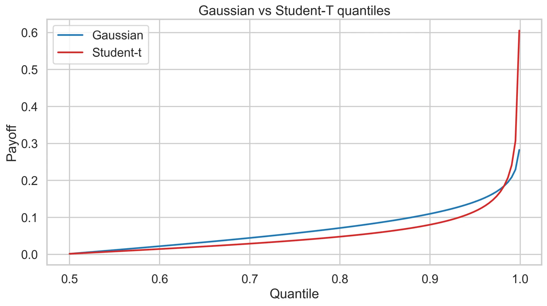
On the chart, the blue Gaussian curve is a bit less aggressive with how it climbs near the end. Inversely, the red Student-t curve goes up and to the right pretty aggressively.

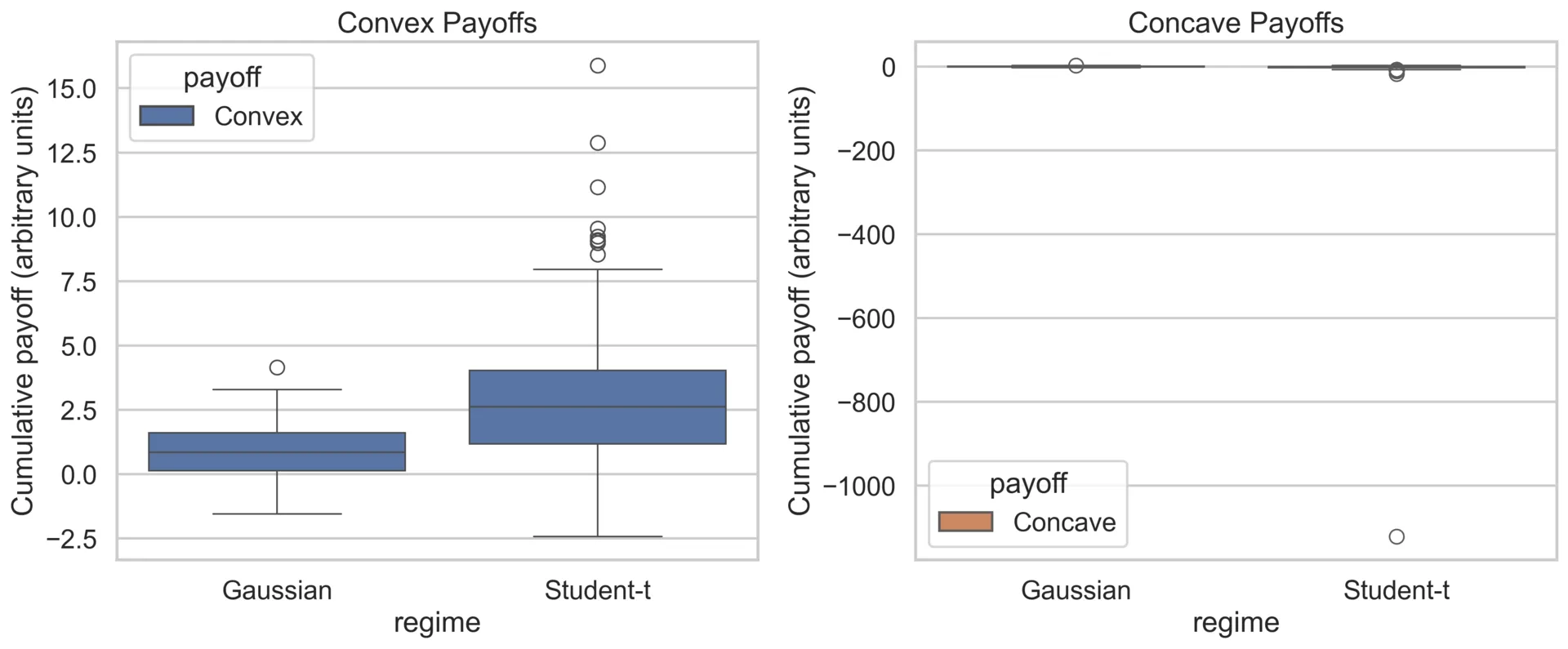
To make the picture concrete, we can take two new toy strategies and see how they would react. A convex payoff that behaves like being long optionality: small moves barely matter, but a huge jump pays off in chunks. And a concave payoff that acts like selling that optionality: you collect pennies until a tail event wipes you out. If we were to input percentiles through those shapes, the convex line shoots upward 🚀 (tail spikes feed it), while the concave one goes real below zero right where our data stopped.

Regime-Shifts Stress Kit

Good backtests will drop in the usual volatile windows (GFC, 2020) or include on a few Gaussian shocks, and while that's a good start it's not nearly enough information to properly model or validate a strategy. Even a 50-year dataset gives you only a handful of true panics, which is nowhere near enough to model how a strategy responds when shocks chain together differently. Rare outliers are the ones deciding whether you're rich or poor, and by definition you don't have enough samples to trust the averages they produce.

A oversimple way to simulate this make a basic regime-shift function that changes the volatility of the fake market and when using the same SMA crossover strategy from before the graph that's produced looks super bad.

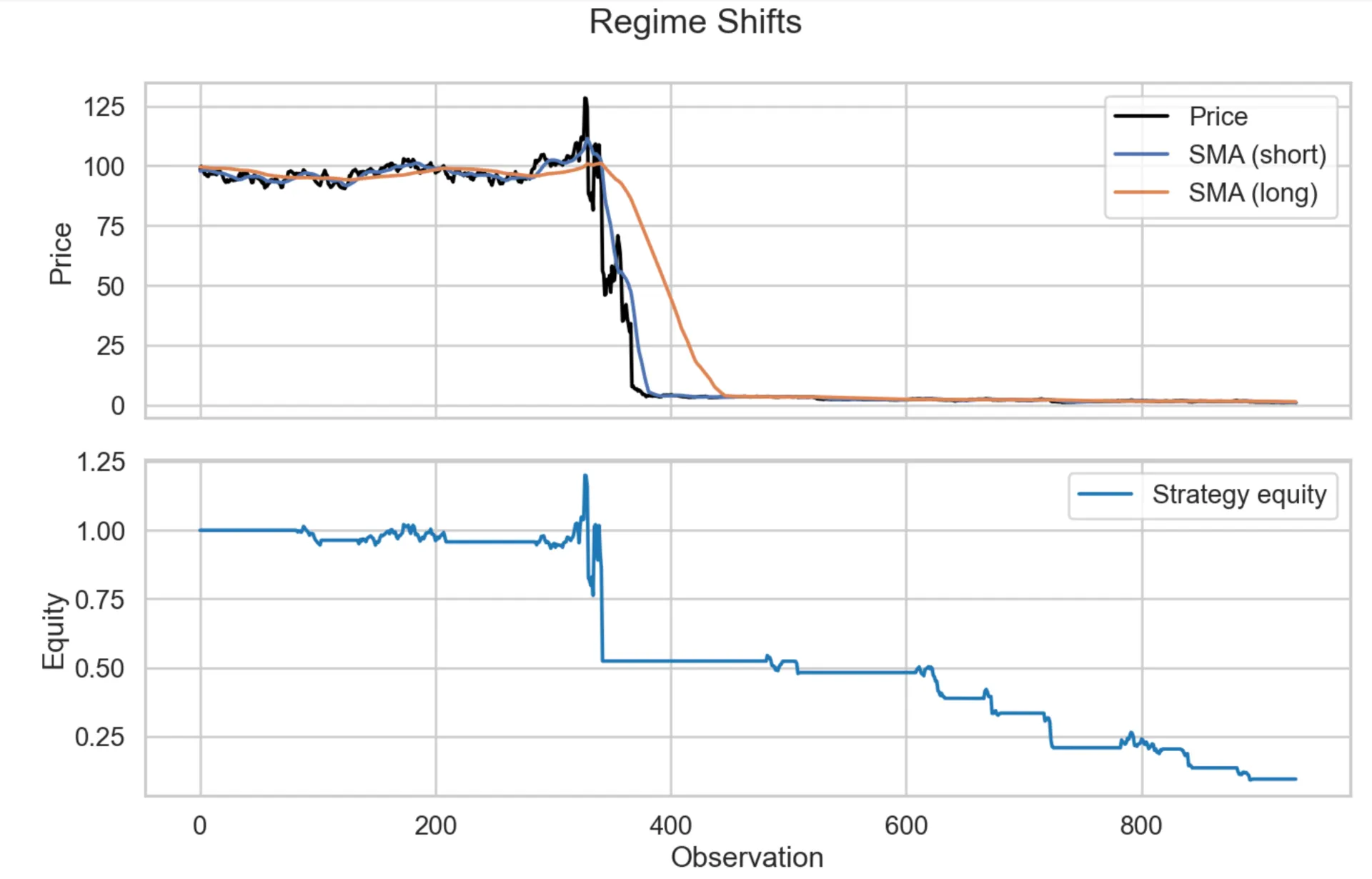
The metrics produced aren't even worth showing because they just suck. The periods of steadiness cause the strategy queue the strategy to do even worse than than all the other market simulation beforehand.

Real-Data Sanity Check with backtesting.py

Enough simulations, let's mess around with some real market data: SPY (daily) and BTC-USD. Let's first what the simple SMA crossover strategy looks like on a couple segmented sections of the market.

real_segments = {
    "SPY": [
        ("Calm 2010-2019", "2010-01-01", "2019-12-31"),
        ("GFC 2007-2009", "2007-01-01", "2009-12-31"),
        ("Pandemic 2020", "2020-01-01", "2020-12-31"),
    ],
    "BTC-USD": [
        ("Rally 2020-2021", "2020-01-01", "2021-11-01"),
        ("Crypto Winter 2021-2023", "2021-11-02", "2023-12-31"),
    ],
}

history_start = {
    "SPY": "2006-01-01",
    "BTC-USD": "2018-01-01",
}

Segment	Total return	Sharpe	Max DD
SPY • Calm 2010-2019	105.0%	0.65	-22.0%
SPY • GFC 2007-2009	11.6%	0.33	-19.8%
SPY • Pandemic 2020	21.2%	1.22	-9.4%
BTC-USD • Rally 2020-2021	467.1%	1.00	-39.5%
BTC-USD • Crypto Winter 2021-2023	35.6%	0.49	-21.2%

So there's way more data in the notebook but it's pretty predictable how this performed. Great for calm periods, bad during crashes like GFC and crypto winter. Someone trading on the assumptions of before the GFC, even if they factored in older crashes like Black Monday in 1987 wouldn't have been able to predict the GFC because there was enough crash data in existence to model it. You could read this and say: "congrats, Johannes. you're just explaining that Black Swans exist. Big deal?" but then perhaps still not understand why backtesting shouldn't give you a lot of confidence. Not all Black Swan event are the same: there's no evidence of blue swans or green swans or anything in between. Likewise "crashes" aren't the same and the takeaway is even with SotA machine learning or the fanciest models out there, there's no way to predict the next crash or what it'll look like.

Better Backtesting & Closing Comments

"Well if backtesting is so bad, then what should you do?" Well, backtesting is fine to do and you shouldn't not use it. You should use it with caution and understand its limitations. Along with backtesting, there's a few additional steps that can help invalidate more strategies:

• Forward test under caps. Run live-but-small with leverage limits and hard stop-loss-on-leverage rules.
• Stress with Pareto tails. Sample shocks from heavy-tailed distributions like Pareto or Student-t instead of just inflating sigma.
• Watch quantiles, not means. Build a simple quantile dashboard (p95/p99 drawdowns, regime-aware VaR) so the tails stay visible.

Further rabbit holes

• Fractal Market Hypothesis and Mandelbrot's argument for Lévy-stable markets.
• Regime-switching models and Hidden Markov Models.
• Agent-based simulations for emergent regime shifts.
• Nonlinear dynamics and chaos in price formation.
• Extreme Value Theory to estimate tail risk.
• Deep generative stress testing for synthesizing adversarial paths.
• I'm basically just a shill for Fat Tails Statistics and thus recommend Taleb's work

Appendix: Beyond Trading

Tail awareness matters anywhere you rely on historical logs. My friend Viraj and his team over at TensorZero (I hope he doesn't mind me flaming him for a sec) just wrote a great blog post on adaptive experimentation using multi-armed bandits (Bandits in Your LLM Gateway). Their Track-and-Stop implementation is well engineered, statistically principled, and, crucially, beats vanilla A/Bs by ~37% in their sims. But while reading it, I couldn't help but notice that every statistical guarantee they rely on implicitly assumes bounded or subgaussian rewards.

The lesson with quant finance is: offline prompt evals ("backtests") are stable only until users drift or a new regime arrives. The bandit layer gives you a live falsification loop, constantly re-testing prompts and reallocating traffic as the surface shifts, which is absolutely the right instinct. But if your reward distribution is fat-tailed, the bandit's confidence bounds can think it’s converging when it’s actually smoothing away the very shocks you care about.

Track-and-Stop's anytime-valid tests are derived under the assumption that rewards are either bounded or have light tails. If your reward metric occasionally throws 50x–100x shocks, the GLRT-based stopping rule can declare a "winner" before the tail risk becomes identifiable.

There are a couple fixes to this problem:

1. Clip or winsorize extreme rewards before feeding them to the bandit loop.

2. Swap the sample mean for heavy-tail-robust estimators: e.g. median-of-means (MOM), Catoni’s M-estimator, trimmed means with adaptive truncation

3. Run a parallel "tail sentry" channel that analyzes the raw (unclipped) rewards with EVT, POT exceedances, stress tests, or change-point detectors.

4. Maintain separate decision layers: i.e. bandit for everyday drift, tail sentry for rare but catastrophic moves

This hybrid setup keeps the bandit fast and reactive while ensuring you don't walk blindly into a 1-in-5,000 spike that corrupts all your estimates.

Fat-Tailed LLM Usecases

1. Whale economics in revenue metrics: Most users give $0–$2, one gives $400. Ergo a single whale makes a mediocre arm look top-tier.

2. Latency with rare catastrophic stalls: 99% of calls: ~0.4s; 1%: ~70s. Ergo means/variances blow up, UCBs become overconfident, and the bandit silently picks an arm with hidden latency bombs.

3. Safety violations with huge negative tails: Mostly safe outputs (reward 0) punctuated by rare –500 violations. Ergo long streaks of “all good” trick the bandit into thinking the arm is safe.

4. Highly skewed few-shot eval scores: Small prompt tweaks yield giant scoring jumps due to semantic edge cases. Ergo heavy Pareto tails invalidate variance-based confidence intervals.

5. Rare user-type catastrophes: A problematic user cohort appears once every ~5,000 requests and interacts badly with a specific arm. Ergo the bandit never sees enough samples to detect the failure.

6. Money-involved credit/refund/bonus systems: Any metric involving dollars tends to be fat-tailed by default. Ergo one anomalous payout distorts the statistics.

7. Hidden long-range dependencies: Rare pathological responses trigger expensive downstream chains (RAG crawlers, agents, tool calls). Ergo true cost appears only hundreds of turns later, violating i.i.d. reward assumptions.